Part 2. Measuring KOI on a Text-to-SQL agent — picking a cost-effective model without dropping quality

In the previous post I introduced KOI (KPI ÷ cost, i.e. outcome per dollar) as a unit for measuring the cost-effectiveness of AI, and Nishiki, a tool that measures it on real data (see the previous post and the Nishiki project page for details). This time I measure it on a task closer to real work. The task is Text-to-SQL: a person asks a question in plain language, the AI writes SQL, queries an internal database, and returns the answer.

The scenario — internal self-service BI

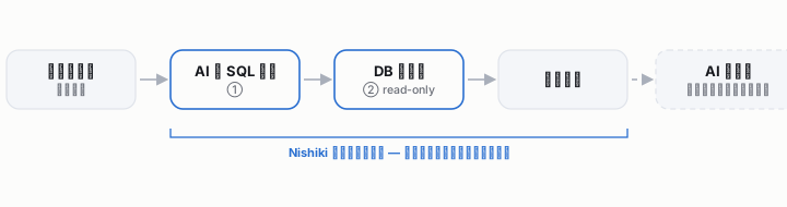
Picture a situation any company has. Sales or management wants to know “what were the top 5 products by revenue in the East region last month?” In the old way, a data analyst wrote SQL each time to answer. Put an AI agent in the middle, and it looks like this:

Person: "Top 5 products by revenue in the East region?"   ← natural language
  ↓  ① AI reads the intent and writes SQL
  ↓  ② the SQL runs on the internal DB → rows come back
  ↓  ③ (if needed) the AI restates the result in natural language
Person: "A, B, C … "

The analyst’s manual work is no longer needed. This is not a one-off chat. As an internal tool it runs automatically thousands to tens of thousands of times a month. That is exactly why both the “smartness” and the “cost” of the model you use matter.

What “AI smartness” means for this task

This is the point I most want to make. Smartness in Text-to-SQL is not general intelligence. It is these three things working together:

1. Reading the intent of the human’s words correctly — what “top 5,” “East region,” and “last month” mean.
2. Understanding the DB schema — which table, which columns, and how to join them.
3. Writing SQL that matches the intent — correct aggregation, filtering, ordering, and joins.

Only when these three come together do you get the right answer. So the smartness to measure is: can the model read the human’s words, build a correct query that matches them, and pull from internal resources properly?

Scoring by “did it actually return the right answer,” not by looks

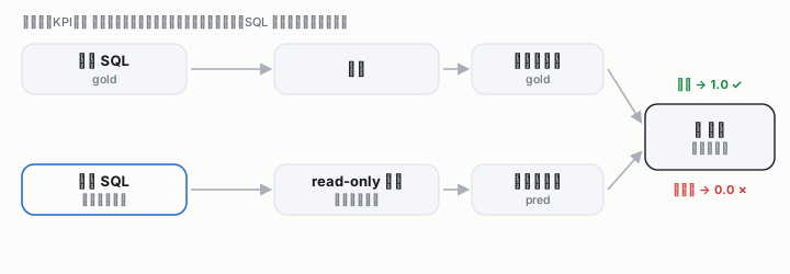
In this sample, Nishiki does not score the text of the generated SQL. It scores whether the rows returned by running that SQL match the correct answer (execution accuracy).

• Different wording is fine as long as the same correct rows come back (price >= 500 and price > 499 give the same result).
• SQL that looks plausible still fails if the result is off.

I think this is scoring that fits real work. What you want is not “good-looking SQL” but “the right numbers.” For safety, execution during scoring always uses a read-only connection, so it never changes the DB.

What KOI shows

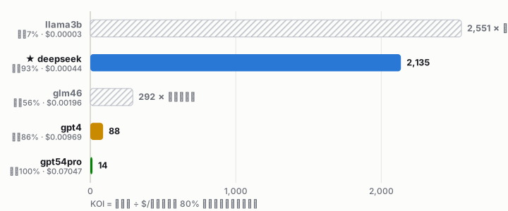
For this run I deliberately used 14 hard questions (window functions, correlated subqueries, anti-joins, HAVING — at the level of real analytical queries) and gave them to five models across a range of prices. The candidates include llama3b, the cheapest small model of them all — the one a plain “cheapest routing” would pick first. I rank by pass rate ÷ cost per item = KOI, but first cut anything below a quality floor (80% here), the “at minimum it must get this right” line.

The table below is measured (14 questions, OpenRouter, about $1.2 total). The routes and unit prices are as written in .nishiki/MODELS.yaml.

Model (route)	Pass rate	Cost/item	KOI	Verdict
llama3b (meta-llama/llama-3.2-3b-instruct)	0.07 (1/14)	$0.00003	2551	✗ cut by floor — cheapest, but only 7% correct
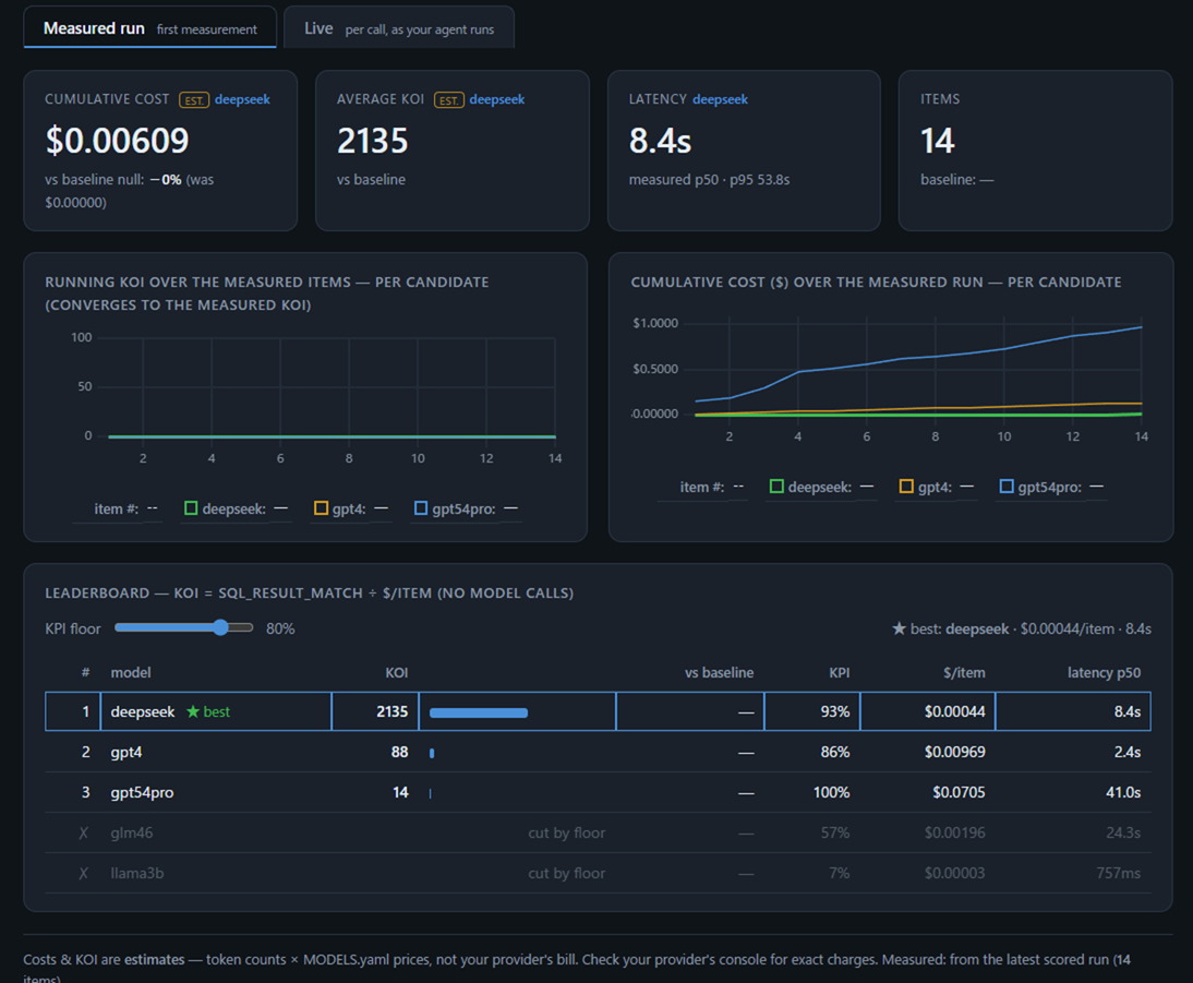
deepseek (deepseek/deepseek-v4-pro)	0.93 (13/14)	$0.00044	2135	★ best value — clears the bar, very low cost
glm46 (z-ai/glm-4.6)	0.57 (8/14)	$0.00196	292	✗ cut by floor — below SLA
gpt4 (openai/gpt-4)	0.86 (12/14)	$0.00969	88	passes, mid-price
gpt54pro (openai/gpt-5.4-pro)	1.00 (14/14)	$0.07047	14	frontier — perfect, but worst value

This table shows the difference between “just pick the cheapest” and KOI.

① The cheapest model has the highest raw KOI, and it is useless in practice. llama3b is nearly free, so even at 7% correct, dividing by a tiny cost makes its KOI the highest at 2551. Rank naively by KOI and it comes out on top. What stops that is the quality floor. 7% is out, of course, and so is glm46 at 57%. Without a floor, “outcome per dollar” would recommend a model that is wrong 93% of the time.

② Among those above the floor, the winner is deepseek — and it is not the cheapest (the cheapest, llama3b, was cut). deepseek wins not on cost but on the ratio of KPI to cost: it clears the 80% bar at 93% while staying at $0.00044, for a KOI of 2135.

③ The frontier model has the highest pass rate (100%) but the lowest KOI (14). For about 160× the cost, it buys only +7 points over deepseek (93→100). Paying that at scale, run after run, is exactly the “cost you can’t justify” that KOI makes visible.

The scatter plot below says it in one image. The vertical axis is accuracy, the horizontal axis is cost (log scale). Anything below the 80% floor line (llama3b, glm46) is grayed out and cut. deepseek sits “above the bar, far left on cost,” and the frontier model sits “at the ceiling, but far right.”

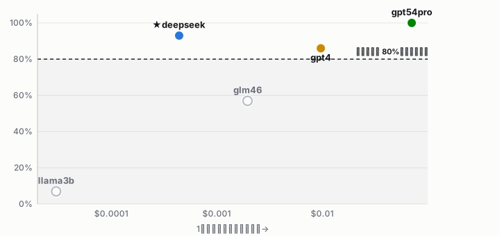
So KOI points to neither the cheapest nor the highest quality. The cheapest (llama3b) is cut by the floor, and the highest quality (frontier) has the worst value. What KOI picks is the one point where, among models above your quality bar, outcome per dollar is highest.

Note that latency is a separate axis from KOI, a reference number not in the formula. Here gpt4 was fastest at about 2.4s and the frontier model slowest at about 41s.

The actual dashboard (the Measured tab of nishiki koi-report --web) looks like this. At the top are cards (cumulative cost, average KOI, latency, count), in the middle a per-item trend chart, and at the bottom a leaderboard with a KPI floor slider. Move the slider and the cut line changes, and the best model swaps in place.

Not just “measure” but “raise” — the optimization loop

Choosing a model is half of optimization. The other half is raising the pass rate with the same model at the same cost, by improving the prompt. Tidy up how you present the schema, add two or three representative example questions, tighten the instructions. This raises the pass rate at unchanged cost, so KOI goes up.

“Lower cost by swapping the model, raise the pass rate by improving the prompt.” These two wheels, before → after, are what it means to optimize the ratio (KOI) rather than just cheapness or just quality. Nishiki updates its baseline every time you measure, so the more you run it the more accurate it gets.

This is not limited to Text-to-SQL — the same holds for RAG and internal-resource use

You will not always use it in exactly this form at work. But the essence can be put this way:

Any use where “the AI reads a human’s intent and pulls the right internal resource” can be measured by KOI with the same framework.

Text-to-SQL is just one case (resource = database, way of pulling = SQL). The same shape appears elsewhere:

• RAG (internal document QA): resource = documents / knowledge base, way of pulling = retrieval + summarization. Score “did it pull the right evidence and answer correctly,” and you can measure the KOI of model choice directly.
• Tool / API-calling agents: resource = internal APIs, business systems, way of pulling = function calls. Score “did it call the right tool with the right arguments.”
• Document matching and extraction (the earlier example from last time): resource = forms, contracts, way of pulling = extraction.

In all of them, the same yardstick — “smartness (= task accuracy) ÷ cost” — lets you measure which model delivers the smartness your use case needs at the lowest price. Only the scoring method changes per task (exact match, execution match, or judgment by another model = LLM-as-judge). Nishiki chooses this scoring from safe built-in parts, so the AI never writes dangerous code on its own.

In short: RAG, Text-to-SQL, or tool calling — any use that has the AI pull internal resources correctly can be measured for cost-effectiveness by KOI and steered toward the best model. The assumption that “smarter equals safer because it costs more” can be re-examined with numbers.

The procedure — getting the best model and KOI with the nishiki command

From here is the actual procedure. The sample is bundled self-contained in the repo (a small synthetic DB, a correct-answer set, and the agent), so you can just run it in order. You never edit the agent’s source. Nishiki only swaps the candidate models in memory during measurement (injection.choke: agent:generate_sql).

The outputs below are the values from actually measuring this sample (14 hard questions, 5 models, OpenRouter, about $1.2 total). The shape of the commands and display stays the same; the numbers change with the models, data, and that day’s prices.

Measuring your own project from scratch — first run and profile generation

This sample comes with its profile, so you can start at step 1 below. But when you measure your own AI project, there is a “first-time setup” and a “profile generation” before that. The whole picture:

nishiki                       # a setup wizard runs the first time only
nishiki init --target <path to your project>   # reads the source and auto-generates a profile
nishiki measure --experiment <the .nishiki created above>   # measures the KPI
nishiki koi-report --experiment <same> --web                # KOI table and best model

① The first nishiki (setup wizard) — the first time you run it, you are asked just three things:

=== Nishiki setup (first run only; no flags needed afterward) ===
[1/3] Choose the orchestrator brain (the LLM that writes the config):
   1) claude_p     [✓ available]      ← the "brain" that writes the config. Choose from claude / codex / OpenRouter / any command
   2) codex        [— not found]
   ...
[2/3] KOI candidate model source:  also list OpenRouter alternatives? [y/N]
[3/3] Data residency policy:  1) stay inside your own cloud (for sensitive data) / 2) unrestricted (include external routes in the comparison)

Your answers are saved and you are not asked again. The “brain” you choose here is the LLM that, in the next init, reads your code and writes out the KPI and candidates automatically.

② nishiki init --target <dir> (profile generation) — it reads the source of the project you point to and, from “what does this agent output,” auto-detects the KPI (choosing a label = classification, pulling text = extraction, building a query = SQL, and so on). Then it creates a .nishiki/ profile right under the target project:

<your project>/.nishiki/
  KOI.yaml       auto-detected scoring recipe (task_type / scorer / floor) + choke (the model-swap point)
  MODELS.yaml    the menu of candidate models (current model + optional OpenRouter alternatives, with prices)
  AGENT.md       a short summary note about the target

It never touches the target’s code, DB, or data (it only adds a hidden tool folder called .nishiki/, which is gitignored). From here, step 1 onward (measure → koi-report) is exactly the same as the bundled sample.

You can measure even on a machine with no “brain.” init’s auto-writing needs one of claude / codex / OpenRouter. But even without one, you can just hand-write .nishiki/KOI.yaml and MODELS.yaml (this sample is exactly such a hand-written profile). measure and koi-report are plain measurement that use no brain at all, so they run on a GPU box or in CI. The only difference is “let the AI write it” vs. “write it yourself”; the measuring part is the same.

Below is the procedure for running this sample, which comes with that hand-written profile.

0. Setup

pip install git+https://github.com/matu79go/nishiki.git    # or: pip install -e . (if already cloned)
cd samples/text_to_sql

If you just want to see the result first, run nishiki koi-report --web at this point and it shows the bundled measured result on the dashboard with no key and no charge (it just replays .nishiki/runs/). Below is the procedure to measure it yourself.

1. Put your key (you can measure for a few cents)

echo 'OPENROUTER_API_KEY=sk-or-...' > .env      # .env is gitignored and never committed

.env is read automatically. An existing environment variable takes precedence.

2. (Optional) Look at the candidate model menu

nishiki models --search deepseek       # pull OpenRouter's live prices with no key

Which models are candidates is written in .nishiki/MODELS.yaml (route slug + price per million tokens). Here I lined up five along a price ladder from frontier down to low-cost, and put the cheapest small model of them all, llama3b, at the bottom. I include it on purpose, in the role of “what plain cheapest-routing would pick.” Deliberately spreading the price range is the point.

Note: I did not auto-pick the candidates for this sample with nishiki models; I chose them by hand. For two reasons. ① Reproducibility — nishiki models pulls the live OpenRouter catalog, so the lineup and prices change by the day. I want the sample to be the same for anyone who clones it at any time, so I fixed the candidates and bundled them. ② A clear point — to show “cheapest ≠ correct,” you need to spread both price and quality on purpose: frontier, mid, low-cost, and a “cheapest but weak” small model. So I added llama3b (cheapest, weak) deliberately. When you measure your own project in production it is the reverse: nishiki init --source openrouter builds candidates by price tier from nishiki models’ live prices (plus the current model extracted from your code). Choosing by hand is only to keep the demo fixed; normal use can be automatic.

3. First, estimate the cost (probe = a small trial run)

Before running everything, try each model on just a few questions to estimate the total cost.

nishiki measure --experiment .nishiki --mode probe --probe-n 3

[probe] in-scope=14 / trial run of 2 items per candidate
  q1 gpt54pro: score=1.00 $0.0705 41000ms
  q1 deepseek: score=1.00 $0.0004 8400ms
  q1 llama3b:  score=0.00 $0.0000 760ms
  ...
  probe actual spend $0.18 / full-run projection $1.20

full-run projection is the estimated cost of the real measurement. If it is unexpectedly high, you notice here.

4. The real measurement (run = score every question × every model)

nishiki measure --experiment .nishiki --mode run

Each model solves all 14 questions, and the generated SQL is run read-only → 1/0 by result match, tallying pass rate and cost per model.

  q1 deepseek: score=1.00 $0.0004 8448ms
  q2 deepseek: score=1.00 $0.0005 5100ms
  ...
[deepseek] KPI 0.93  NGrec -  $0.0061($0.00044/item) err=0
[llama3b]  KPI 0.07  NGrec -  $0.0004($0.00003/item) err=0
...
→ .nishiki/runs/<stamp>_run.json
  next: nishiki koi-report --experiment .nishiki

The results are saved in .nishiki/runs/*.json (the info to re-measure with the same models next time is also kept in last_run.json).

5. Output the best model and the KOI table (this is the goal)

nishiki koi-report --experiment .nishiki --web

KOI dashboard ready  (recommended: deepseek)
  → http://127.0.0.1:8765/#measured

The recommended model prints in the terminal and the KOI dashboard opens in the browser. The table is ordered “first cut by the floor (the lower bound on pass rate) → then the survivors by KOI (pass rate ÷ cost), descending.” The floor is a slider, so change the SLA — say “I must hold a 90% pass rate” — and you can watch the best model swap in place. (To print just the table in the terminal without a browser, drop --web.)

6. (Optional) See the per-item breakdown

nishiki history --experiment .nishiki

For each question, you can check one by one which model produced what SQL, whether it was right, how many tokens, and how much it cost.

7. (Optional) Live KOI — measure while it runs

nishiki run --experiment .nishiki --fresh --watch -- \
  python agent.py "How many products cost 500 dollars or more?"

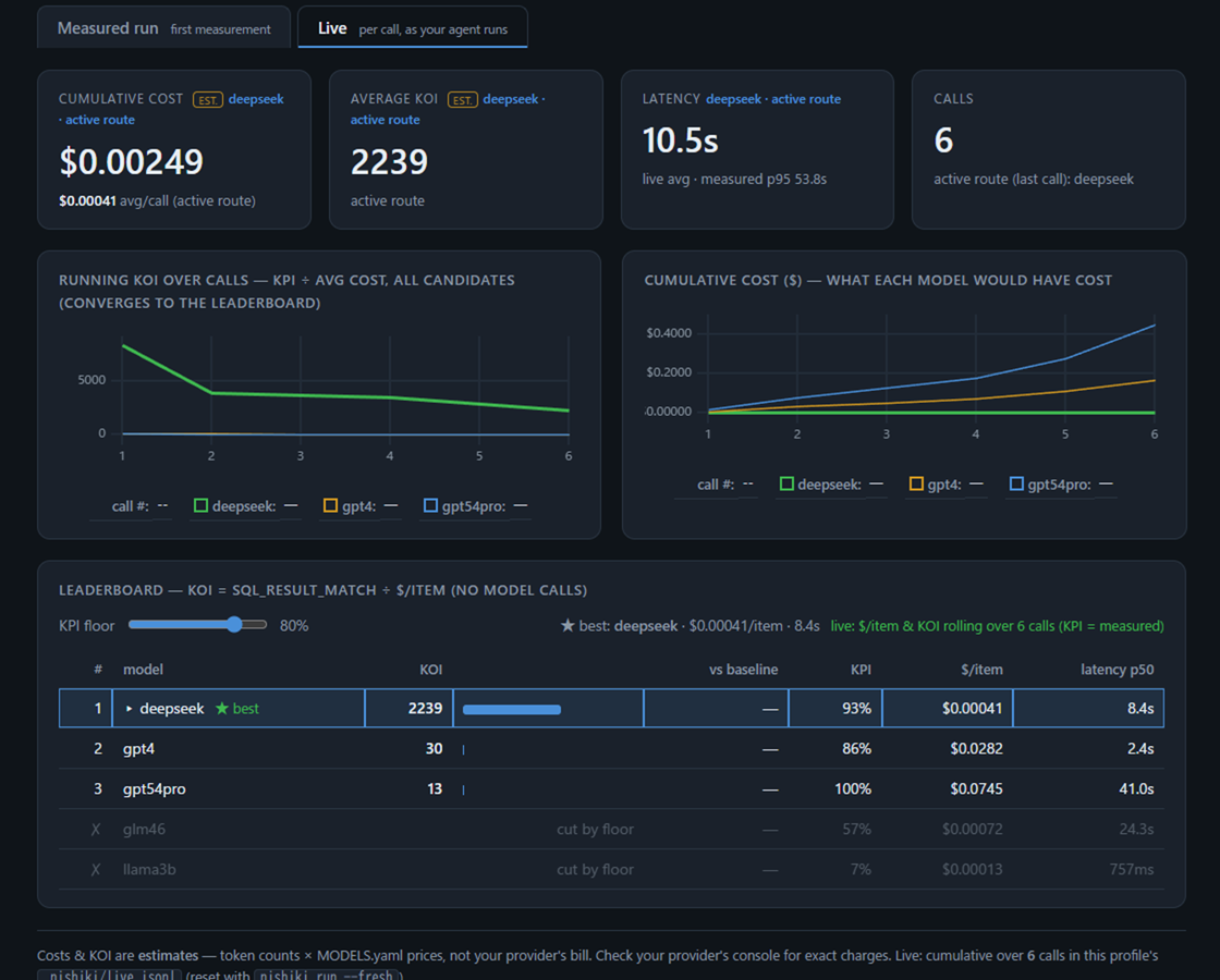
It wraps the agent along with its launch command and, by reading the real tokens of each call, shows KOI as it goes (with no extra API calls). When you connect to a production agent, this one command gives you live measurement too. On the dashboard’s Live tab, KOI and cumulative cost move with each call, and all candidates re-rank on a rolling basis by measured $/item.

8. “Raise” KOI — the optimization loop

Once the best model is set, next you raise the pass rate with the same model at the same cost. Just improve run.prompt in .nishiki/KOI.yaml (for example, add two or three representative questions with model-answer SQL) and re-measure.

# Edit run.prompt in .nishiki/KOI.yaml, then…
nishiki measure --experiment .nishiki --mode run
nishiki koi-report --experiment .nishiki --web       # check pass rate↑ → KOI↑ before/after

Raise or lower the floor (floors.kpi_floor) to match your work’s SLA, and you can re-pick “the best-value model among those that meet that quality line.”

9. Leave it all to the tool

Even without memorizing the steps, you can just type nishiki in this directory. The orchestrator guides you interactively from init to measurement to the KOI table (and replies in your language).

---

(Prices are OpenRouter list prices = USD per million tokens, pulled live with nishiki models. Pass rates and costs are the bundled measured values. The numbers change with the models and data you measure. The DB is entirely fictional, domain-neutral synthetic data.)